Run a conceptual model

In this tutorial, we demonstrate how to run a conceptual hydrological model using torchHydroNodes.

Before we start

This tutorial is rendered from a Jupyter notebook that is hosted on GitHub. If you’d like to run the code yourself, you can access the notebook and configuration files directly from the repository: 01-RunConceptModel Tutorial.
To run this notebook locally, ensure you have completed the setup steps outlined in Getting started. These steps include setting up the environment, installing the required packages, and preparing the data files necessary for the tutorial.

Import packages

[12]:

%reload_ext autoreload
%autoreload 2

import sys
from pathlib import Path
from tqdm import tqdm

# Dynamically set the project directory based on the notebook's location
notebook_dir = Path().resolve()
project_dir = str(notebook_dir.parent.parent)  # Adjust based on your project structure
sys.path.append(project_dir)

from src.thn_run import (
    _load_cfg_and_ds,
    get_basin_interpolators
)

from src.modelzoo_concept import get_concept_model

from src.utils.log_results import (
    save_and_plot_simulation,
    compute_and_save_metrics,
)

from tutorials.utils import (
    display_run_plots
)

Constants

[13]:

config_file = 'config_run_concept.yml'

Load config file and prepare dataset

[14]:

cfg, dataset = _load_cfg_and_ds(Path(config_file), model='conceptual')

-- Loading the config file and the dataset
-- Using device: cpu --
Setting seed for reproducibility: 111
-- Loading basin dynamics into xarray data set.
  0%|          | 0/4 [00:00<?, ?it/s]100%|██████████| 4/4 [00:00<00:00, 10.31it/s]

[15]:

cfg._cfg['experiment_name']

[15]:

'run_concept_model'

A folder has been created in the runs directory with the name specified as experiment_name in the configuration file, appended with a YYMMDD_HHMMSS timestamp. This folder will contain the configuration, results, plots, and metrics associated with the run.

Explore cfg file and created dataset

[16]:

# Inputs taken from the config file and generated as needed
cfg._cfg.keys()

[16]:

dict_keys(['dataset', 'concept_data_dir', 'forcings', 'basin_file', 'concept_model', 'ode_solver_lib', 'odesmethod', 'time_step', 'train_start_date', 'train_end_date', 'valid_start_date', 'valid_end_date', 'metrics', 'experiment_name', 'device', 'seed', 'precision', 'verbose', 'config_dir', 'basin_file_path', 'concept_inputs', 'concept_target', 'periods', 'run_dir', 'plots_dir', 'results_dir', 'number_of_basins'])

[17]:

# Dataset attributes
dataset.__dict__.keys()

[17]:

dict_keys(['cfg', 'is_train', '_compute_scaler', 'scaler', 'basins', '_disable_pbar', '_per_basin_target_stds', '_dates', 'start_and_end_dates', 'num_samples', 'period_starts', 'alias_map', 'alias_map_clean', 'ds_train', 'ds_valid', 'ds_static'])

[18]:

display(
    'basins', dataset.basins,
    'start_and_end_dates', dataset.start_and_end_dates,
    'ds_train', dataset.ds_train,
    'ds_valid', dataset.ds_valid,
)

'basins'

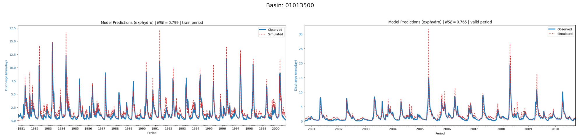
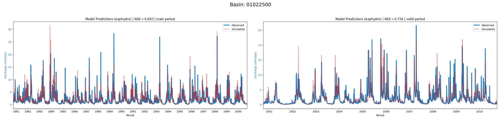
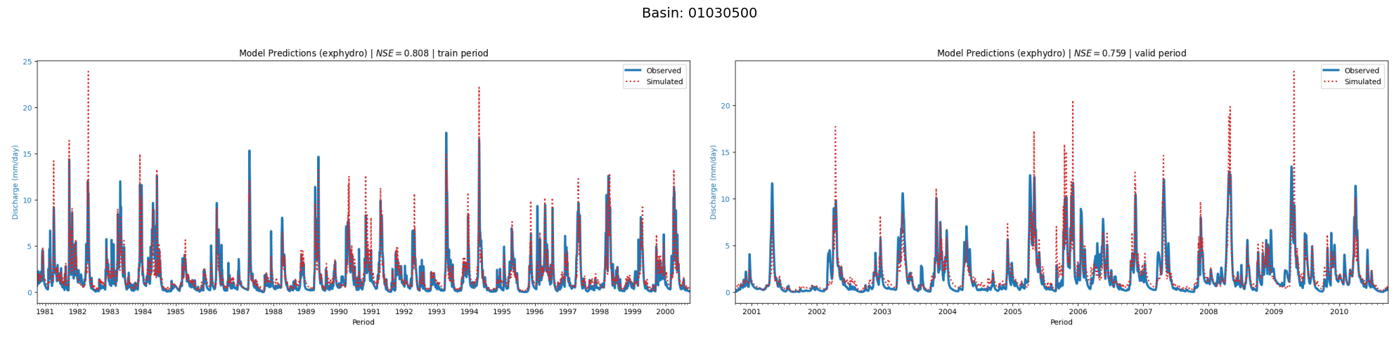
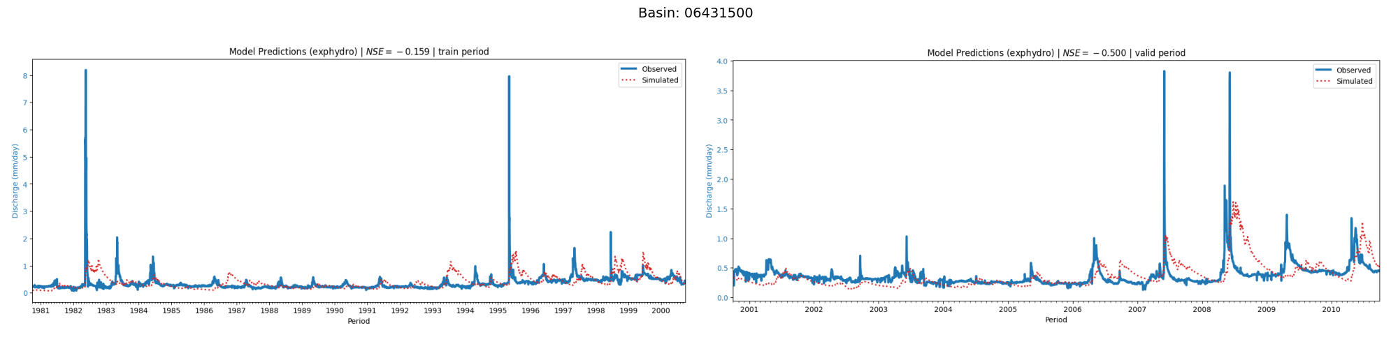
['01013500', '01022500', '01030500', '06431500']

'start_and_end_dates'

{'train': {'start_date': Timestamp('1980-10-01 00:00:00'),
  'end_date': Timestamp('2000-09-30 00:00:00')},
 'valid': {'start_date': Timestamp('2000-10-01 00:00:00'),
  'end_date': Timestamp('2010-09-30 00:00:00')}}

'ds_train'

'ds_valid'

Feel free to generate plots from the training and validation sets to get familiar with the data

Create interpolators

As the time-series data was loaded on a one-day resolution, we need to run interpolation during the solution of the system of ODEs for adaptative-step methods and fixe-step methods with higher resolution.

[19]:

# Get the basin interpolators
interpolators = get_basin_interpolators(dataset, cfg, project_dir)

Run the model and save the results

[20]:

for basin in tqdm(dataset.basins, disable=cfg .disable_pbar, file=sys.stdout):

    for period in dataset.start_and_end_dates.keys():

        if period in ['train', 'valid']:
            if period == 'train':
                time_idx0 = 0
                data = dataset.ds_train
            else:
                time_idx0 = len(dataset.ds_train['date'].values)
                data = dataset.ds_valid

            model_concept = get_concept_model(
                cfg, data, interpolators, time_idx0, dataset.scaler, odesmethod=cfg.odesmethod
            )
            basin_data = data.sel(basin=basin)

        # Update Initial states for the model if period is not 'train'
        if period != 'train':
            model_concept.shift_initial_states(dataset.start_and_end_dates, basin, period=period)

        # Run the model
        model_results = model_concept.run(basin=basin)

        if model_results is None:
            continue

        # Save the results
        model_concept.save_results(basin_data, model_results,
                                   basin, period=period)

        # Plot the results
        save_and_plot_simulation(ds=basin_data,
                            q_bucket=model_results[-1],
                            basin=basin,
                            period=period,
                            model_name=cfg.concept_model,
                            plots_dir=cfg.plots_dir,
                            plot_prcp=False
                        )

  0%|          | 0/4 [00:00<?, ?it/s]100%|██████████| 4/4 [00:18<00:00,  4.61s/it]

Test the model (compute metrics)

[21]:

run_dir = cfg.run_dir

# After the model has been run for all basins and periods
# Evaluate the model - Compute the metrics
compute_and_save_metrics(metrics=cfg.metrics, run_dir=run_dir)

Load plots

[22]:

# Example usage
display_run_plots(
    basins=dataset.basins,
    periods=list(dataset.start_and_end_dates.keys())
)

Latest folder: runs/run_concept_model_241202_160120

../_images/tutorials_run-concept-model_21_1.png

../_images/tutorials_run-concept-model_21_2.png

../_images/tutorials_run-concept-model_21_3.png

../_images/tutorials_run-concept-model_21_4.png